Modeling Multivariate Longitudinal Factors on HIV Patients Cell Counts at Gonder University Specialized Hospital, Ethiopia

Department of Statistics, College of Computing and Informatics, Haramaya University, P.O.Box: 138, Dire Dawa, Ethiopia

^*Corresponding author: Alebachew Abebe, Department of Statistics, College of Computing and Informatics, Haramaya University, P.O.Box: 138, Dire Dawa, Ethiopia; Email: [email protected]

Received Date: May 6, 2024

Publication Date: July 17, 2024

Citation: Abebe A. (2024). Modeling Multivariate Longitudinal Factors on HIV Patients Cell Counts at Gonder University Specialized Hospital, Ethiopia. Mathews J Surgery. 7(2):32.

Copyright: Abebe A. © (2024)

ABSTRACT

Modeling of multivariate longitudinal data provides a unique opportunity in studying the joint evolution of multiple response variables over time. This study was modeling of multivariate longitudinal data cell counts on HIV infections at Gondar districts were used two different multivariate repeated measurement with a kronecker product covariance and random coefficient mixed models. The study was based on data from 566 per four visits HIV infections were enrolled in the first 4 visits of the 5-year secondary data with retrospective study design. Both models of HIV infections cell counts values of CD4 and CD8 increase over time while hemoglobin decreases over time. Those models results reveals that a strong positive correlation between CD4 and CD8 cells, but the correlation between CD4 and hemoglobin as well as the correlation between CD8 and hemoglobin are not statistically significant. Consequently, the study suggests that concerned bodies should focus on awareness creation to increase cell counts of CD4 and CD8 over time while hemoglobin decrease over time for HIV infections at Gondar districts, Ethiopia.

Keywords: HIV Infections, Cell Counts, Multivariate Longitudinal Data, Kronecker Product Covariance, Random Coefficients

INTRODUCTION

Longitudinal data consist of repeated measurements that belong to same subjects/units. This type of data might arise in many research fields such as medical sciences [1-4]. The repeated measurements are typically dependent and these dependencies (associations) must be taken into account to have valid statistical inferences [5].

Longitudinal data are often collected on multiple responses. In such a case, in addition to the within-subject association, two additional association structures, multivariate response association at a specific time point and cross-temporal response association, occur. The multivariate responses could either belong to the same response family or different response families. In literature, there are two common approaches to handle multivariate longitudinal data rather than jointly analyzing them. First one is to ignore the multivariate response association and construct univariate models [6] or carry out univariate cluster analyses [7,8]. The second one is to consider one of the responses as the dependent variable and the other(s) as independent one(s) together with the other independent variables and to construct a univariate model [9].

From the clinical point of view, what is required for the present model is that an essential component of the immune system is the Lymphocytes which destroy invaders. Lymphocytes are of two types B-cells and T-cells, being B-cells antibody factories producing antibodies as fast as they can and also clone themselves, whereas T-cells either direct the activity of B-cells (called CD4+T-cells) or act as suppressors (called CD8+T-cells) destroying infected cells and thus damp out the activity of the immune system. The AIDS has three stages, one including the initial infection, a second one of latency and the third one corresponding to a runaway destruction of the immune system. During the latency lapse healthy T-cells are infected although its number remains high. When the concentration of T-cells decreases and that of HIV virus cells increases, it is the AIDS stage. In practice, as an example, cytometry is a procedure useful to count the concentration of healthy, latently infected and infected T-cells in the blood stream, for instance using the dispersion of laser light, which depends on the enzymes covering the cells [23]. Knowing the concentration of CD4+T-cells it is possible to wonder about modeling the evolution of the different cell populations. Among the various models trying to describe the dynamics of CD4+T-cells (see for instance [24, 25]), a simple one describing the phases of latency and the destruction of the immune system is Perelson’s model [26, 27, 28].

A total of 566 per four visits (2264 individuals) were enrolled in HIV infections for this study and followed up to 5-years with in 4 repetitions. In this study, we only considered modeling of multivariate longitudinal response variables for HIV infections have three responses. These are CD4 counts (CD4), CD8 counts (CD8) and Hemoglobin levels (HMG). Our primary interest was to assess the inter-relationships among these multivariate responses. For an easy notation, throughout this study we let X, Y, and Z represents for CD4, CD8 and HMG respectively. We note that, as ubiquitous in longitudinal studies, not all multivariate responses are measured at all occasions in HIV infections data. In spite of their practicability, these approaches do  not yield valid statistical inferences. In this study, we consider the accommodation of the afore-mentioned three association structures with a multivariate modeling approach for multiple responses belonging to the same response family.

However, the analysis of such a modeling of multivariate longitudinal data can be challenging because (i) the variances of errors are likely to be different for different subjects, (ii) the errors are likely to be correlated for the same subjects measured at different occasions, and (iii) the errors are also likely to be correlated among subjects measured at the same time. In the SAS software, 2 different approaches have been provided to analyze modeling of multivariate longitudinal data: modeling of multivariate repeated measurement models with a kronecker product covariance structure [15] and random coefficient mixed models [12].

In this study, we first present the HIV infections data that motivates our study. Then we illustrate and compare these 2 approaches in studying the joint evolution of the modeling of multivariate longitudinal data for HIV infections at an early stage of HIV infections data. The objectives of this study was to explore the joint evolution of CD4 counts, CD8 counts and hemoglobin levels of HIV infections and to compare modeling of multivariate repeated measurement models (kronecker product covariance and random effects mixed model) using HIV infections data of North Gondar, Ethiopia. In this study, model development procedures were Akaike Information Criteria (AIC), Bayesian Information Criteria (BIC) and Likelihood Ratio Test (-2LnL).

MATERIALS and METHODS

Study Area and Data Descriptions

This study was based on data from 566 per four visits (2264 individuals) persons with HIV infections were enrolled in the first four visits of the five year multivariate longitudinal study of HIV infections using the data of North Gondar, Ethiopia. The study design was retrospective on multivariate longitudinal data setting that go back in time to compare multivariate repeated measurement models with a kronecker product covariance structure and random mixed effects model and to explore the joint evolution of CD4, CD8 counts and hemoglobin levels of HIV infections. The secondary data were collected from different part of North Gondar districts that measured repeatedly in four visits between the years on May 30, 2013 to May 30, 2017. Each repeated measures were conducted on the average six month interval in the study period. In this study all multivariate longitudinal data response variables were time variant and independents variables were time variant and invariant.

Eligible Criteria

Outstanding to some natural and unknown reasons few person fail to continue up to the end of the study period. This study was considered both inclusion and exclusion criteria.

Inclusion Criteria

Throughout the data collection, we were selected person who have HIV infections that could have four repeatedly measured over time data were included in the study period. That is, the repeatedly measured data with four follow-ups (visits) person with HIV infections were included in the study.

Exclusion Criteria

HIV infections who dropout (withdraw), intermittent missing values and loss to follow-up within the study period was excluded from the study. Hence, person who may have died from other cause, refuse and others who do not participate at the previous measurement (attrition) time of the study period was excluded from the study. Although, the time period before May 30, 2013 and after May 30, 2017 HIV infections would been excluded from the study.

Variables Considered in the Study

HIV infections were considered as multivariate longitudinal data act as the response variables. That variable has three categories were CD4 counts, CD8 counts and hemoglobin levels even if they were used as a continuous variable to maximize the amount of information available in the data set.

The independent variables such as cite of HIV infections (Chilga, Debark, Gondar and Metema), ART number, visits (1^st, 2^nd, 3^rd & 4^th), and value of HIV infections and time of HIV infections were included in the study. The first two variables were used for descriptive statistics and the remaininng variables were applied for inferential statistics (modeling part).

Methods of Statistical Analysis

Multivariate longitudinal data is a special case of repeatedly measured data, the observations are not independent and are characterized as having both between-subject and within-subject variation, time dependent covariates and missing data [10]. Furthermore, multivariate longitudinal data response variables have become increasingly popular, more accessible and good in missing data handling through statistical software such as SAS Virson-9.4 [13].

Exploring Data Analysis

Exploring the Correlation Structure

Each covariance model has a corresponding correlation model. Even though there are so many models for covariance structure. There are 4 types of covariance models were considered and compared in this study [29].

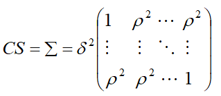
Compound Symmetry (CS)

Suppose that a parameter representing the common correlation for any two time points, then the correlation here,  where the single correlation parameter  is generally referred to as the intra-class correlation coefficient.

Let us assume that, with m repeated measures.

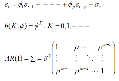
Autoregressive Order One (AR(1))

Autoregressive models express the current observation as a linear function of previous observations plus a homoscedastic noise term, α_t , centered at (E[α_t] = 0) and assumed independent of the previous observations.

Toeplitz (TOEP)

If there were m measures, then there will be two distances: one unit distance, two units distance. And, hence two parameters were estimated.

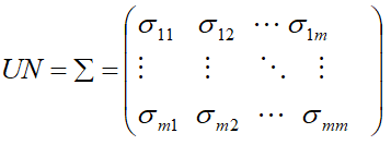
Unstructured (UN)

Unstructured covariance matrix allows m different variances, one for each time point and   distinct off-diagonal elements representing the possibly different covariance for each pair of times, for a total of  variances and co-variances.

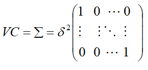
1. Simple (VC): The simple model assumes independent observations and homogeneous variance. This is the default. 
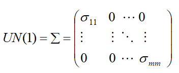
2. UN (1): Different variance and 0 covariance. 

Model Selection

It is one of a most series problem in data analysis. The variance-covariance structure with the lower AIC, BIC and likelihood ratio test (-2LnL) value can be an appropriate to select the model. Most commonly in epidemiological studies, investigators frequently attempt to construct the most desirable statistical model using the popular methods of forward, backward, and stepwise regressions [30].

Intra-Cluster Correlation (ICC)

The covariance matrix of the random-effects is thought to summarize the ICC. If there are a large number of random-effects components, then this leads to a complex covariance matrix and can increase computational burden [31].

Multivariate Repeated Measurement Models

Kronecker Product Covariance Structure

The first approach considered is to fit a model with a kronecker product covariance structure. This model allows investigator to specify the variance-covariance matrix of the measurement error within each study unit (i.e., subject) and thus to examine the intra-and inter-subject correlations of the measurement errors. The data layout for this model has the following presentation, where the variable VISIT indicates that all the assessments are equally spaced while the variable TIME gives the exact measurement time (six month). Where, PHID stands for patient who have HIV infections identified card in the SAS program. To assure normality and homoscedasticity of the residual distribution, the response variable is defined as the change in value of subject at time t since the initial visit, i.e.,

Table 1: The data layout presentation for multivariate longitudinal of HIV data.

Proc mixed data=HIV_MIX covtest noclprint;

Title1 “model 1 mixed model with a kronoker product covariance”;

Title2 “CD4 (X) versus CD8 (Y)”;

Class PHID vname visit;

Model value=vname*visit/s noint;

Repeated vname visit/ type=UN@AR(1) subject=PHID r rcorr;

Where vname=“CD4” or vname=“CD8”;

Run;

The option TYPE=UN@AR(1) in the REPEATED statement specifies that the covariance matrix with in an individual has the following structure:

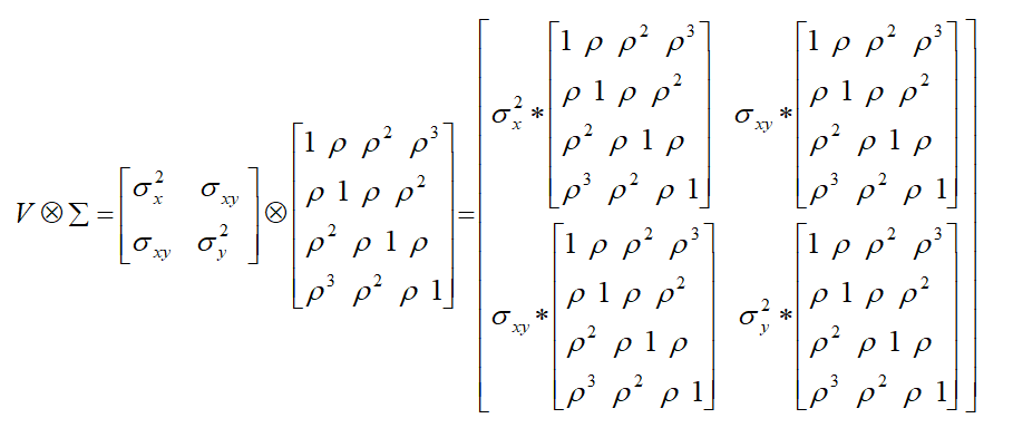
Thus, the above model assumes that (i) the two cells (CD4 & CD8) share a common intra-cells correlation as measured by:

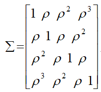, and (ii) the inter-cells correlations (as measured 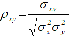) are the same for two cells measured at the same time point. The two cells are independent if the matrix V has the form of 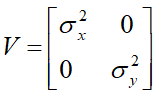, and the hypothesis H₀: σ_xy = 0 will be tested by the COVTEST option.

Random Coefficient Mixed Models

Instead of modeling the variation with in the study unit as in the repeated measurement models, the random coefficient mixed models assume that the regression coefficients are a random sample from some population of possible coefficient and allow one to model variations between study units [14]. In the presence of multiple response variables, a separate set of regression coefficients will be fitted for each response variable and the correlations among these random coefficients can be examined. In SAS this model is also implemented with PROC MIXED and the data layout of the model is exactly the same as in previous section. The following SAS codes fit a random coefficient mixed model for CD4 and CD8. We note that the variable TIME rather than VISIT is used in the model, indicating its capability to handle equally spaced measurements. The syntax/program in SAS version-9.4 was fitted the random coefficient mixed models were presented below.

Proc mixed data=HIV_MIX covtest noclprint;

Title1 “model 2 mixed model with random coefficients”;

Title2 “CD4 (X) versus CD8 (Y)”;

Class PHID vname;

Model value=vname*time/s noint;

Random vname*time/ type=UN subject=PHID g gcorr;

Repeated / type=VC group=vname subject=PHID;

Where vname=“CD4” or vname=“CD8”;

Run;

The RANDOM statement requests that two random slopes (one for CD4 and one for CD8) be fitted for each individual and the GROUP option in the REPEATED statement specifies that the variances of measurement errors are different for different cells. The G and GCORR options in the RANDOM statement require the display of covariance and correlation matrix for the random slopes respectively, with 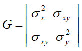, the two slopes are independent if σ_xy = 0.

RESULTS

Among the total of 566 per four visits (2264 individuals) HIV infections data at North Gondar Zone, Ethiopia for category of CD4 counts were 852(37.6%), while in CD8 counts were 644(28.4%) and the remaining hemoglobin levels were 768(33.9%) presented in figure-2 and table-2. However, figure-1 revealed that the value of HIV infections data at North Gondar Zone, Ethiopia was approximately skewed to the right direction or decrease to the right direction.

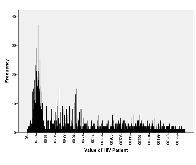
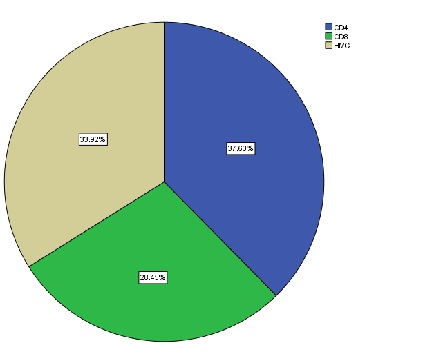
Figure 1: Bar-chart for value of HIV  Fig. 2: Pie-chart for variables name of HIV distribution.

In table-2 reveals that each visit of HIV infections per visits were 566(25%). According to this scenario in HIV infections of the cite Chilga have 1016(44.9%), Debark cite have 84(3.7%), Gondar cite have 456(20.1%) and the rest HIV infections have 708(31.3%) in Metema cite.

Table 2: Categorical variables of HIV infections data (n=566)

Table 3: Cross-tabulation for visit on variables name of HIV infections data.

Table 4: Continuous variables of HIV infections data at North Gondar Zone, Ethiopia (n=566).

The results show that, patients with HIV infections, the values of CD4 and CD8 increase over time while hemoglobin (HMG) decreases over time. All these changes are significantly different from zero (with P<0.001 for CD4 and CD8, P<0.05 for HMG respectively). The results also reveal that a strong positive correlation between CD4 and CD8 cells (ρ_X,Y=0.463 with P<0.001), but the correlation between CD4 and HMG (ρ_X,Z, P=0.148) as well as the correlation between CD8 and HMG (ρ_Y,Z, P=0.217) are not statistically significant. We note that these correlations index had the extra associations among cell counts after removing the effect of involution process over time.

Table 5: Bivariate mixed models with a kronoker product covariance on HIV infections data.

The results of mixed models with random coefficients are listed in table-6 where the slope parameter represents the average change per six month for each cell counts over time. For simplicity, only the estimated correlation coefficients out of the random effect portion are listed in table-6.

Results show that CD4 and CD8 increase over time (P<0.001) while HMG decrease (P<0.05). There exist a strong positive correlation between CD4 and CD8 (ρ_X,Y=0.753 with P<0.001), but the correlation between CD4 and HMG (ρ_X,Z=-0.074, P=0.536) as well as the correlation between CD8 and HMG (ρ_Y,Z=-0.045, P=0.764) are not statistically significant. However, it should be pointed out that the correlation coefficients in table-6 represent the associations among random slopes (i.e., the trajectory of cell counts over time) rather than measurement errors. We also note this approach is easily extendable to multivariate longitudinal data with more than two response variables.

Table 6: Heterogeneous mixed models with random coefficients on HIV infections data

DISCUSSIONS

In this study was conducted comparison of the 2 approaches for multivariate longitudinal data modeling: the 2 different approaches considered in this study to explore different aspects of the joint evolution of multiple response variables, and thus each approach has its own advantages and limitations.

The first models with kronecker product covariance provide a convenient way to fit bivariate data and enable one to examine both inter-cell and intra-cell correlations of the measurement errors. However, this model possesses several apparent limitations, namely, a common intra-cell correlation for different cells, a constant inter-cell correlation for cells measured at the same time point, as well as the demanding for equally spaced measurements. Furthermore, SAS only provides the possibility to fit bivariate mixed models.

The second models with random coefficients provide an opportunity to examine correlations among the trajectories of cell counts over time and to capture the growth of these response variables. As exemplified by the HIV data, this approach is capable of handling equally spaced measurements and is easily extendable to multivariate models with more than two response variables. Another advantage of these mixed-model approaches is that they allow incomplete observations and thus can use information more efficiently.

CONCLUSION

According to this study in the early stage of HIV infections, CD4 and CD8 steadily increase over time while the values of hemoglobin (HMG) decrease over time. There exists a strong positive correlation between the two cell counts of HIV infections. The correlations between the cell counts (CD4 and CD8) and hemoglobin levels are not significant in either measurement errors or random slopes, but CD4 and CD8 cells show a negative cross-lagged effect on hemoglobin levels, i.e., the higher the value of CD4 (CD8) at time t-1, the lower the hemoglobin measurement at time t.

DECLARATIONS/ ETHICAL STANDARDS

Ethical Approval and Consent to Participate

Ethical clearance had been obtained from Department of Statistics at Haramaya University, Dire Dawa, Ethiopia.

Consent for Publication

This manuscript has not been published elsewhere and is not under consideration by another journal. Author has approved the final manuscript and agreed with its submission to Archives of Public Health. I agreed about authorship for this manuscript.

Availability of Data and Materials

I used secondary data for this investigation obtained at University of Gonder Teaching and Specialized Hospital.

Competing Interests

The authors declare that he has no competing interests.

Funding

No applicable!

Author Contributions

Author wrote the proposal, developed data collection format, supervised the data collection process and analyzed the data in consultation with Mr. Gashaw A. MSc in Public Health. He is also edited the document and gave critical comments. Author read and approved the final manuscript.

Acknowledgments

In a special way, I wish to extend my sincere gratitude to Mrs. Elesabet G. for her support and guidance accorded me during this study. I would also like to acknowledge the contribution of my colleagues from whom I enjoyed fruitful discussion on challenging topics.

Author’s Information

Alebachew Abebe is an Assistant Professor of the department of Statistics at Haramaya University, Ethiopia, He had previous eight manuscripts and one proceeding.

REFERENCES

1. Hoefield RA, Kalra PA, Baker PG, Sousa I, Diggle PJ, Gibson MJ, et al. (2011). The use of eGFR and ACR to predict decline in renal function in people with diabetes. Nephrol Dial Transplan. 26:887-892.
2. Taylor-Robinson D, Whitehead M, Diderichsen F, Olesen HV, Pressler T, Smyth RL, et al. (2012). Understanding the natural progression in % FEV1 decline in patients with cystic fibrosis: a longitudinal study. Thorax. 67: 860-866.
3. Yates JW, Watson EM. (2013). Estimating insulin sensitivity from glucose levels only: use of a non-linear mixed effects approach and maximum a posteriori (MAP) estimation. Comput Methods Programs Biomed. 109:134-143.
4. Jang H, Conklin DJ, Kong M. (2013). Piecewise nonlinear mixed-effects models for modeling cardiac function and assessing treatment effects. Comput Methods Programs Biomed. 110:240-252.
5. Zeger SL, Irizarry R, Peng RD. (2006). On time series analysis of public health and biomedical data. Annu Rev Public Health. 27:57-79.
6. Shelton BJ, Gilbert GH, Liu B, Fisher M. (2004). A SAS macro for the analysis of multivariate longitudinal binary outcomes. Comput Methods Programs Biomed. 76:163-175.
7. Genolini C, Falissard B. (2011). KmL: a package to cluster longitudinal data. Comput Methods Programs Biomed. 104:112-121.
8. Genolini C, Pingault JB, Driss T, Côté S, Tremblay RE, Vitaro F, et al. (2013). KmL3D A non-parametric algorithm for clustering joint trajectories. Computer Methods and Programs Biomedicine. 109:104-111.
9. Weiss RE. (2005). Modeling Longitudinal Data. Springer-Verlag, New York.
10. Davis CS. (2002). Laird NM, Ware JH. (1982). Verbeke G, Molenberghs G. (2009). Statistical Methods for the Analysis of Repeated Measurements. New York: Springer Verlag.
11. Laird NM, Ware JH. (1982). Random-effects models for longitudinal data. Biometrika. 38:963-974.
12. Verbeke G, Molenberghs G. (2009). Linear Mixed Models for Longitudinal Data. New York, NY: Springer.
13. Singer JD. (1998). Using SAS Proc Mixed to fit multilevel models, hierarchical models, and individual growth models. J Educational Behavioral Stat. 23:323.
14. Littell RC, Milliken GA, Stroup WW, Wolfinger RD. (1996). SAS System for Mixed Models, Cary, NC: SAS Institute Inc.
15. Thiebaut R, Jacqmin-Gadda H, Chene G, Leport C, Commenges D. (2002). Bivariate linear mixed models using SAS proc MIXED. Comput Methods Programs Biomed. 69:249-256.
16. Newsom JT. (2002). A multilevel structural equation model for dyadic data. Structural Equation Modeling. 9:431-447.
17. Galecki AT. (1994). General class of covariance structures for two or more repeated factors in longitudinal data analysis. Communications in Statistics-Theory and Methods. 23:3105-3119.
18. Chapman AB, Guay-Woodford LM, Grantham JJ, Torres VE, Bae KT, Baumgarten DA, et al. (2003). Renal structure in early autosomal-dominant polycystic kidney disease (ADPKD): the Consortium for Radiology Imaging Study of Polycystic Kidney Disease (CRISP) cohort. Kidney Int. 64:1035-1045.
19. Henderson CR. (1984). Applications of Linear Models in Animal Breeding. Guelph Canada: University of Guelph Press.
20. Gurrin LC. (2005). Solving mixed model equations. New York: John Wiley and Sons. 120:120-142.
21. MacCallum R, Austin JT. (2000). Application of Structural Equation Modeling in psychological research. Annu Rev Psychol. 51:201-226.
22. Hatcher L. (1998). A step-by step approach to using the SAS System for factor analysis and structural equation modeling, Cary, NC: SAS Institute Inc.
23. Ormerod MG. (2008). Using the dispersion of laser light, that depends on the enzymes covering the cells of HIV infection. Flow Cytometry (Garland Pub.).
24. Murray JD. (2002). Mathematical Biology I. An Introduction to multivariate longitudinal data. (Ed. Springer).
25. Perelson S, Weisbuch G. (1997). Immunology for physicists. Rev Mod Phys. 69:1219-1267.
26. Perelson AS, Kirschner DE, De Boer R. (1993). Dynamics of HIV infection of CD4+ T cells. Mathematical Biosciences. 114:81-125.
27. Perelson S, Nelson PW. (1999). Mathematical analysis of HIV-1 dynamics in vivo. SIAM Rev. 41:3-44.
28. Perelson AS. (2002). Modeling viral and immune system dynamics. Nat Rev Immunol. 2:28-36.
29. Diggle PJ. (2002). Analysis of Longitudinal Data, 2nd ed. New York: Oxford University Press.
30. Hosmer DW, Lemeshow S. (1989). Applied Logistic Regression. New York: John Wiley and Sons, Inc:376-381.
31. Peng H, Lu Y. (2012). Model selection in linear mixed effect models. J Multivariate Anal. 109:109-129.